How to Train Your Own Decision Model With Minimal Changes to an LLM
We trained a 4B LLM to be a decision model on one A100 by changing very little, since a decision model is a glorified classifier. This guide shows how, with every number from our runs.
We trained a 4B LLM to be a decision model on one A100 in under three days. Training took its one-pass readout from 62.7% to 72.5%, and with thinking reserved for its least certain questions, it gets 81.8% of our 5,442 eval questions right at 729 thinking tokens per question.
That took very little change to the model, because decision models are glorified classifiers. They read text and pick among labels, and a pretrained LLM already carries the internal states to make that call, so all it needs is to learn to decide in the language of your labels. That is why we kept the base weights and LM head frozen, let LoRA adapters do the learning, added no new head, and read every answer from the option-label logits.
That idea became a category only two months ago. TypeSafe launched Jev on September 15, and within weeks there was an open-weight answer from Cloudflare, a “thinking” decision model from Fastino, a 421M encoder from an independent researcher that crossed 19,000 GitHub stars in five days, and a community leaderboard with more than 170 entries. That pace is why so many teams want their own, and why most writing on training one is still a launch post or a model card.
TL;DR: Change a strong small LLM as little as you can: freeze the base and LM head, train LoRA so it reads option probabilities from its own label logits in one pass, calibrate on held-out data, and route only the least certain questions to thinking. Data drove most of our gains, and 60 steps of RL repaired the thinking that chain training had hurt while cutting thinking tokens by more than half.
Both models are open weights on Hugging Face, each with a full model card: the 4B, decision-model-qwen3.5-4b, and the 2B, decision-model-minicpm5-2b-lora.
What Is a Decision Model?
A decision model takes a state (a ticket, an email, a tool call, a JSON record) and a set of typed questions about it, and returns a probability for every possible answer, with no generated text. That makes it a classifier whose labels arrive with each request, and most models use Jev’s names for the three question types: choice picks one option from a list, score places the state on an ordered scale, and noul is a yes/no question that returns a single probability.
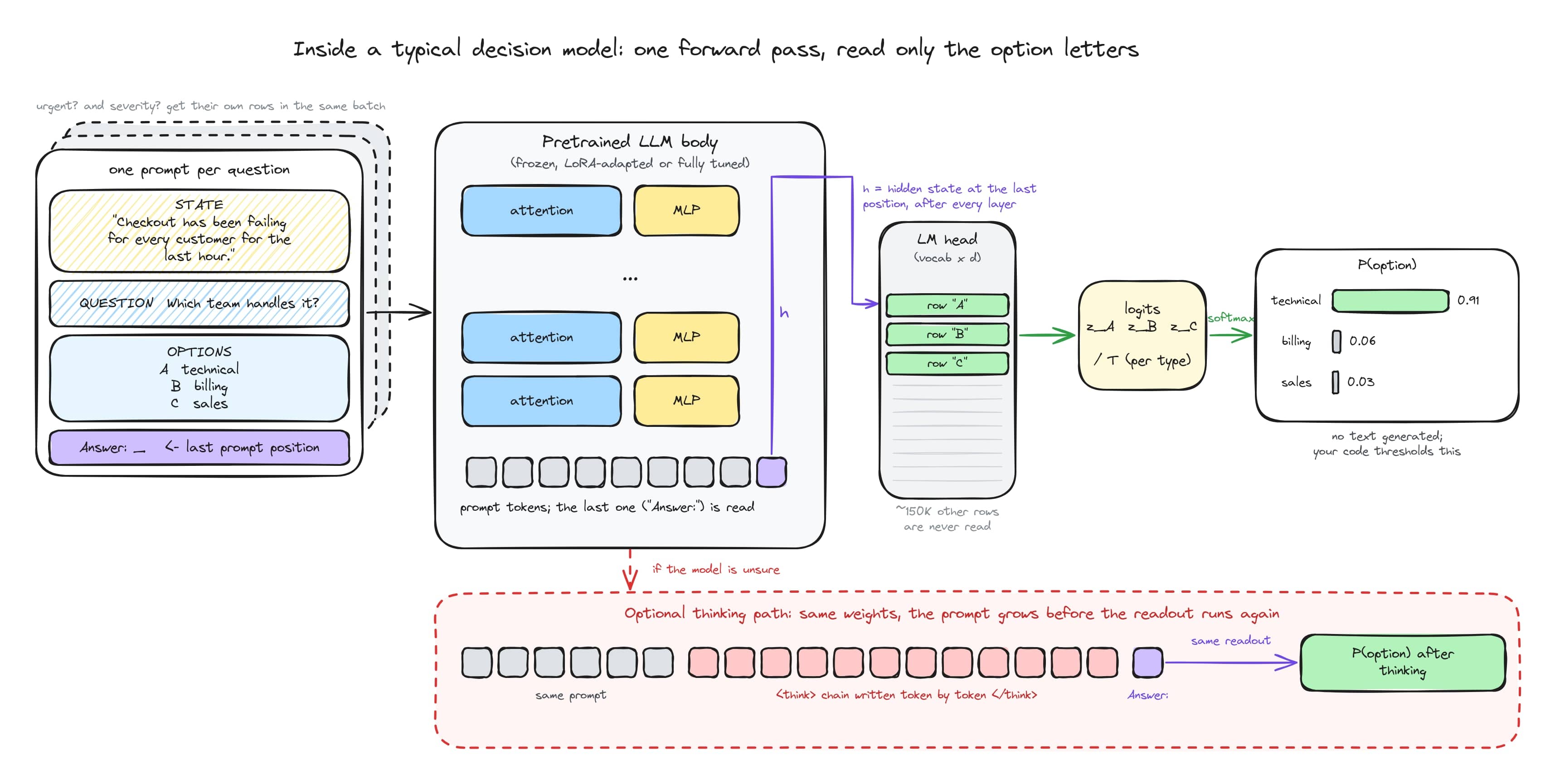
A pretrained LLM already reads labels from a prompt, so many decision models are just that LLM with a very narrow output. The prompt holds the state, one question and its letter-labeled options, and one forward pass yields logits for only those letters at the last position, which a softmax with a fitted temperature turns into probabilities. The LM head already has a row for every letter, so this readout adds no parameters. Models that think write a chain first and then run the same readout, while Laya and Clef add a small head of their own.
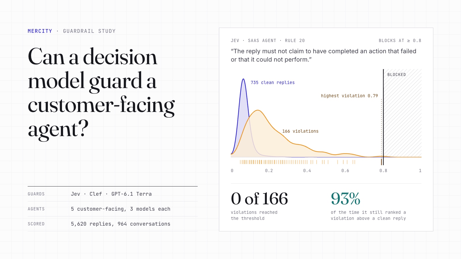
Because the output is a probability over options you defined, it works like a smart if-statement: your code blocks, routes or escalates on the number, and the model cannot return an unoffered label or malformed JSON. It is also cheap: Jev charges $0.042 per million input tokens and nothing for output, against $0.20 to $10 per million for general LLMs. We compared them with classifiers and LLM judges in our post on using decision models as security guardrails.
Should You Train Your Own Decision Model?
That low price is why most organizations should not start by training, since a hosted model is a few lines of code and good enough for generic routing or triage. Training pays off only when three things hold at once: you make the same kind of decision at high volume, the decision depends on your own policies or data, and that data cannot leave your network.
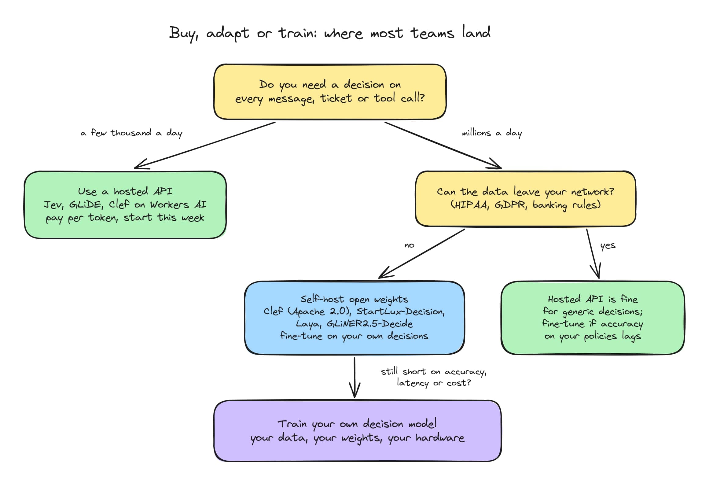
Compliance is usually what tips it. A hospital routing patient messages under HIPAA, or a bank scoring transactions under GDPR and local banking rules, often cannot send that state to a third-party API. Open weights solve part of this, since Clef is Apache 2.0 and StartLux-Decision ships open models from 0.8B to 27B with vLLM, llama.cpp and MLX builds. Owning the training pipeline closes the rest: you choose the data, retrain when policies change, and can show an auditor exactly how the model was built.
Decision Model Recipes That Emerged Since Jev
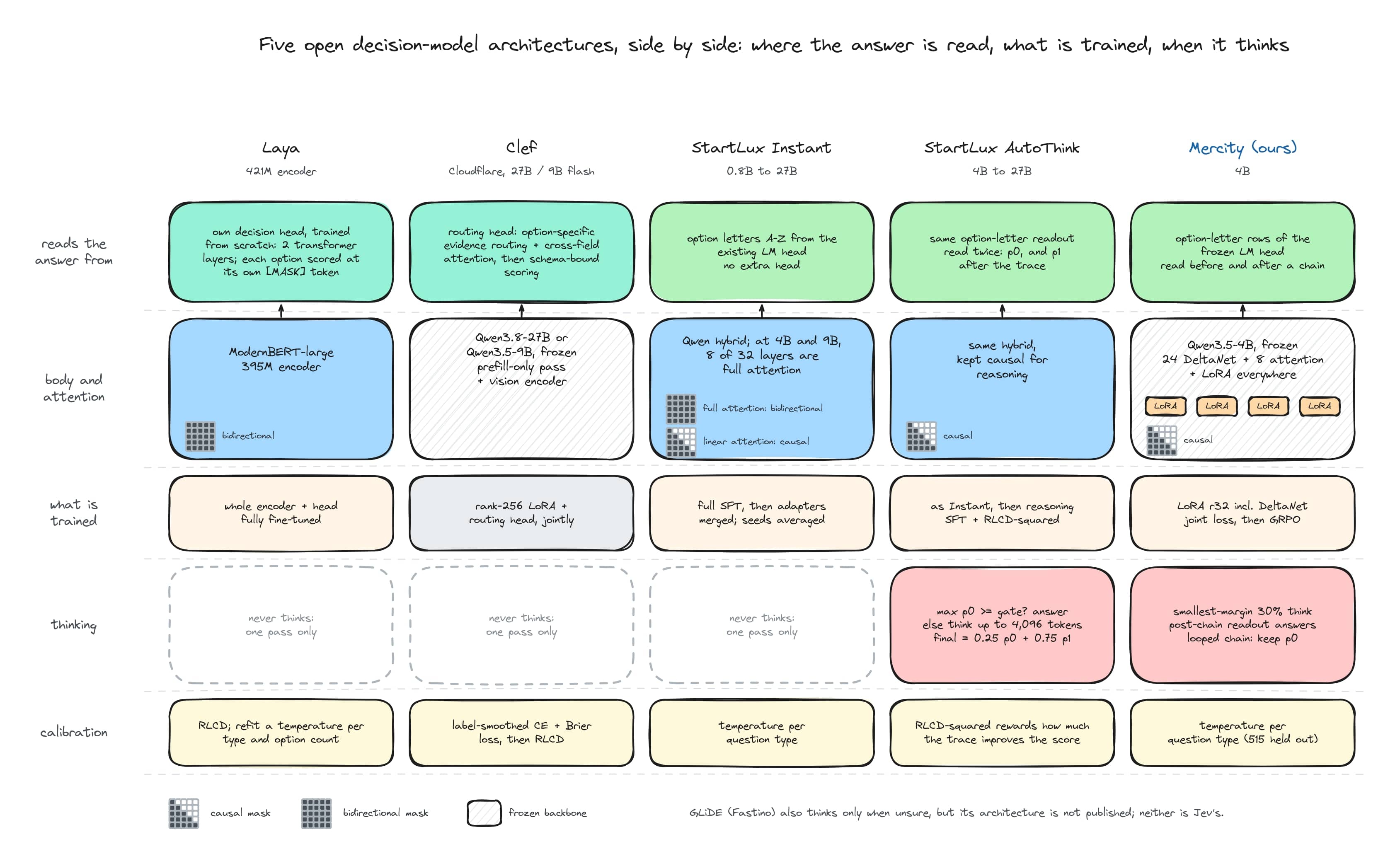
Training no longer means starting from zero. TypeSafe never published Jev’s procedure, so the community worked it out in public, and four approaches keep recurring. They differ mostly in how much they change the backbone, from new heads and full fine-tunes down to a bare label readout, and in how they handle hard questions.
Readouts on Top of an LLM Backbone
The most common recipe reads the answer from a pretrained LLM’s internal states in one prefill pass. Cloudflare’s Clef freezes a Qwen backbone (Qwen3.8-27B for Clef, Qwen3.5-9B for Clef-flash) and trains rank-256 LoRA adapters jointly with a routing head that lets each option gather its own evidence from the prompt before scoring. Label-smoothed cross-entropy plus a Brier loss keeps those scores calibrated. StartLux’s Instant models change the backbone instead, making the full-attention layers bidirectional so every option sees the whole prompt.
We used its lightest form, with no head, because you inherit everything the LLM knows and serve it on the stack you already run.
Small Encoders You Fine-Tune on Your Own Decisions
Laya took the opposite bet: a 421M ModernBERT-large encoder with one mask token per option, answering in about 33 ms. Zero-shot it is close to chance on the independent typed-decisions benchmark (0.36), but after fine-tuning on 1,200 cases from that benchmark it reaches 0.766 accuracy against Jev’s 0.727, at roughly a fifth of Jev’s latency.
So a small model trained on your decisions can beat a frontier decision model on your task, provided you fix its calibration. Laya’s own model card says the checkpoints ship over-confident, and one temperature per question type and option count takes the English model’s mean ECE from 0.466 to 0.081. An independent reproduction found the opposite, an under-confident checkpoint (ECE 0.214) that one held-out temperature brought to 0.037. When sources disagree even on the direction of the error, calibrate whatever you train yourself.
RLCD and Proper Scoring Rules
Calibration is also what Jev’s training method targets. Reinforcement Learning for Calibrated Decisions (RLCD) rewards a strictly proper scoring rule, such as the log or Brier score, which a model maximizes only by reporting honest probabilities. Laya, Clef and StartLux all use some version of it.
That popularity deserves skepticism. The maintainers of exu-base, an open RLCD toolkit, report that in fourteen comparisons on real data, directly optimizing the proper score was as good as or better than RLCD. We took the simpler route, training our readout with plain cross-entropy against target distributions and fitting temperatures afterwards.
Decision Models That Think When Unsure
The newest direction removes the trade-off between fast and careful by reasoning only when unsure. Fastino’s GLiDE was the first to ship this, and StartLux’s AutoThink models think only when the top probability falls below a gate, 0.6 by default in their repo, 0.9 in the paper’s evaluations. Their RLCD 2 method rewards reasoning by how much it improves the decision probabilities, with a penalty on long traces, and cuts average reasoning length by up to 65%.
One model can then cover cheap routine decisions and the occasional one that needs arithmetic or several rule checks, which is the design we built ours around.
How We Trained Our Own Decision Model
We set out to build a Jev-style typed decision model that could also think, and to do it on hardware a mid-sized team can rent: a single A100 80GB, from October 30 to November 1, 2026. All code, data, logs and checkpoints are in our public Hugging Face bucket, and both final models are released as open weights: the 4B and the 2B.
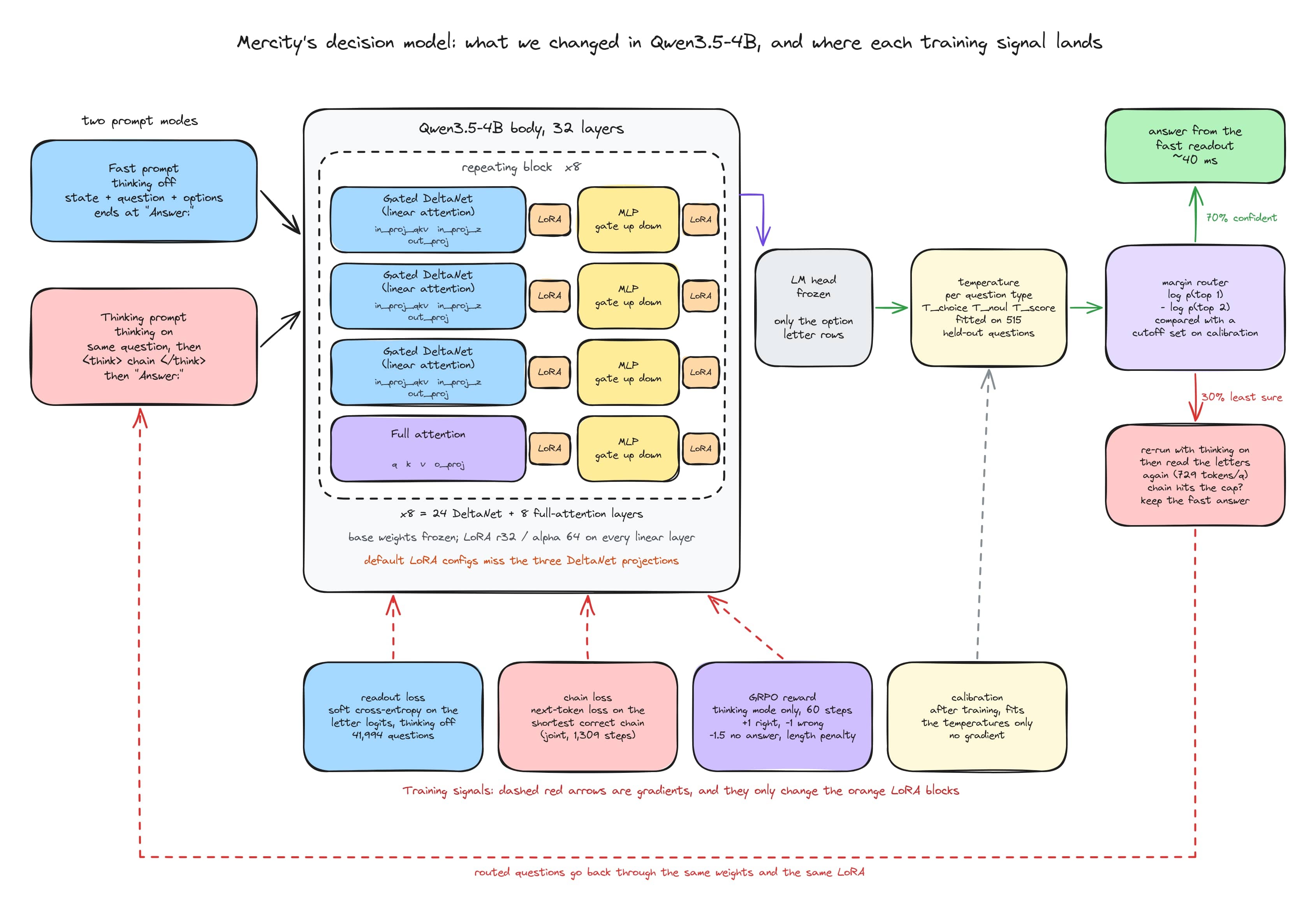
The result is one model with two modes. The fast readout restricts the next token to the option letters and reads their probabilities in one pass, in about 40 ms. Thinking mode writes a reasoning chain and then reads the same letters, so a router can answer from the fast readout and send only the least certain questions to thinking.
That needed very little architectural change, which is this post’s thesis in practice. The base weights and LM head stay frozen, LoRA adapters sit on every linear layer, and calibration and routing live outside the network, so they can be refit without touching the weights. Six steps built it.
Step 1: Probe the Base Model Before You Commit
Every later step depends on the backbone, so first probe it: run each untouched candidate on your own questions before spending GPU hours on training. We ran the zero-shot fast readout on all 5,442 eval questions and four thinking chains each on 128 training questions, in one short loop (simplified from probe_models.py):
for model in ["Qwen/Qwen3-4B", "Qwen/Qwen3.5-4B"]:
    llm = load_in_vllm(model)
    # Test 1: zero-shot fast readout, one forward pass per eval question
    report["readout_acc"] = accuracy_by_set(readout(llm, eval_questions))
    # Test 2: thinking mode, 4 chains each on 128 training questions
    chains = think(llm, train_pool[:128], n=4)
    report["first_chain_acc"] = share_correct(first_of(chains))
    report["median_chain_tokens"] = median(c.tokens for c in chains)
    report["parse_rate"], report["looped"] = parse_rate(chains), count_loops(chains)
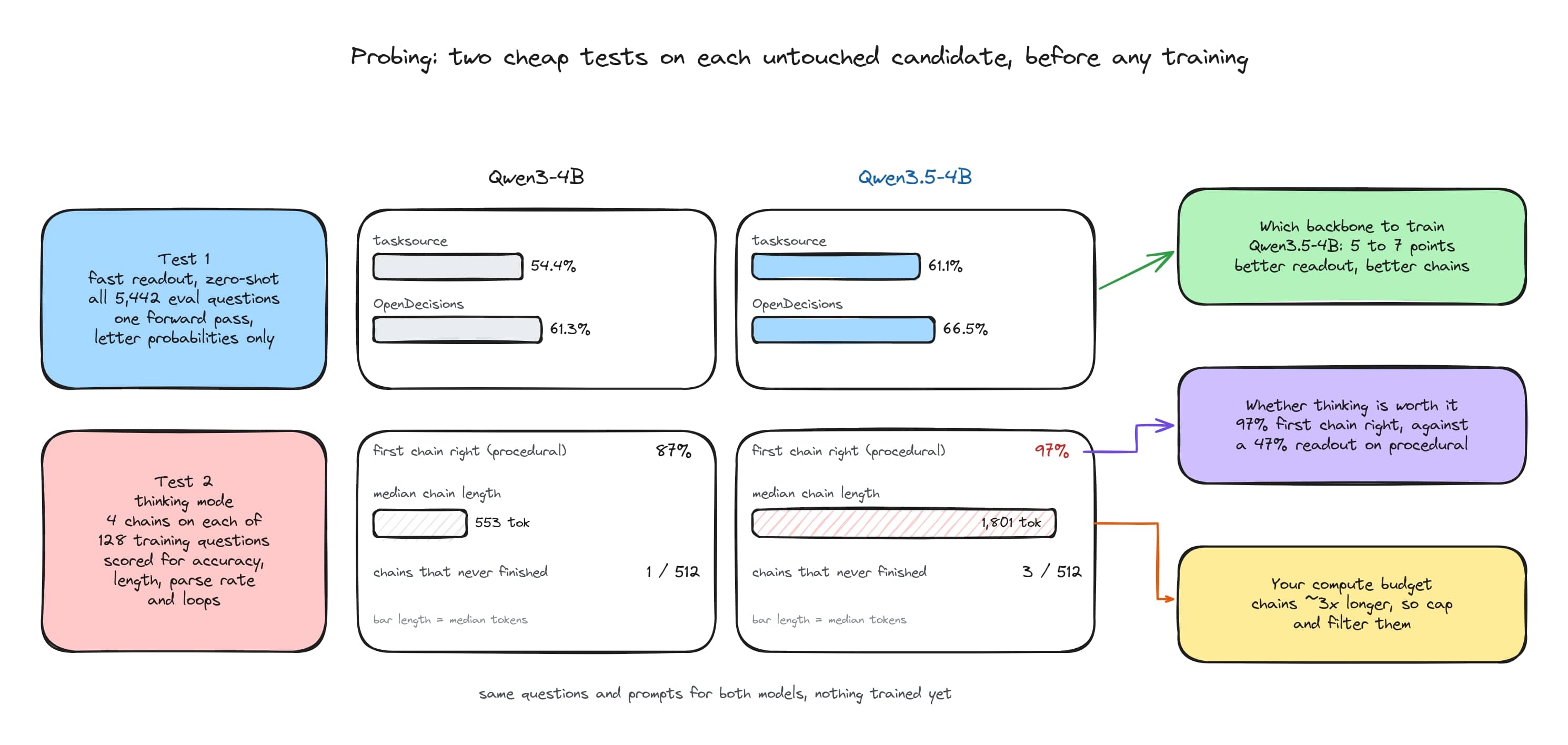
That loop changed our plan. We expected to use Qwen3-4B, but Qwen3.5-4B was 5 to 7 points better on the fast readout for natural-language sets, and its first chain was right 97% of the time on procedural tasks against 87%. The probe also showed the cost: chains about three times longer (median 1,801 tokens against 553), which set every compute budget after that.
The switch also changed what LoRA had to touch. Qwen3.5-4B is a hybrid whose 24 of 32 layers are Gated DeltaNet linear attention, and default LoRA configs target only standard attention and MLP projections, so we also put rank-32 LoRA adapters on the linear-attention projections. On any hybrid, check which modules your adapters touch. Our LoRA guide covers the basics.
Step 2: Build Training Data That Covers the Whole Space
With the backbone fixed, the question became what to teach it. Our final training set had 41,994 readout questions: 18,000 procedural questions from generators with exact labels (tables, budgets, schedules, rule checks), and 23,994 questions converted from 717 tasksource datasets. Half were shown in the option order the eval uses, so the model would not learn to favor positions.
Thinking mode also needed chains, and the probe had warned they would be long. We sampled four per question and kept only the shortest correct one, which cut median chain length on tasksource from 1,662 to 734 tokens, and dropped chains where fewer than 2 of 4 samples were right, chains that nearly looped, and chains claiming to remember the dataset (“I found a similar question online”). For 662 hard questions the 4B rarely solved, we bought chains from Qwen3.5-35B-A3B through OpenRouter for $6.60 in total.
That effort paid off, because data was our biggest lever: going from 3K to 42K readout questions took the fast readout from 69.5% to 72.7%. One idea backfired, since mixing gold labels with the model’s own vote shares as soft targets made the readout 1.2 points worse, so train on reliable labels directly.
Step 3: Train the Readout and the Reasoning Together
Since one model serves both modes, one LoRA adapter trains on both kinds of example, mixed in the same batches. A readout example is the question with thinking off, scored by soft cross-entropy between the option-letter softmax and the target distribution. A chain example is the question with thinking on plus the shortest correct chain from Step 2, scored by next-token loss. In train.py it reduces to:
readout_example = {"kind": "readout", "prompt": question_thinking_off,
                   "target": {"A": 0.0, "B": 1.0, "C": 0.0}}    # gold label as a distribution
chain_example   = {"kind": "chain", "prompt": question_thinking_on,
                   "completion": shortest_correct_chain + answer_letter}

if ex["kind"] == "readout":
    z = lm_head[option_letters] @ hidden[answer_position]       # one logit per option letter
    loss = -(target * log_softmax(z)).sum()                     # soft cross-entropy
else:
    loss = mean_next_token_ce(chain_tokens)                     # ordinary language-model loss
We chose the learning rate with a three-way sweep and a rule written before seeing results: the lowest rate within 0.01 dev NLL of the best. That gave 2e-4, and fixing the rule first stops anyone quietly picking the run that looks best on eval. The final run trained 1,309 steps on 47.8M tokens in 2 hours 46 minutes.
Step 4: Calibrate Before You Set Any Threshold
A trained readout is useful only once 0.9 means right about 90% of the time, because every production threshold depends on it. We fitted one temperature per question type on 515 held-out calibration questions, never eval data, bringing the final fast readout’s expected calibration error to 0.030.
Good calibration can still hide a bias. Our model said yes 62% of the time on yes/no questions where gold was yes 50% of the time, and one logit offset fitted on calibration data lifted balanced accuracy from 78.4% to 83.6% in distribution. On an outside benchmark the same offset helped some tasks and hurt as many, so recalibrate on data from the domain you deploy into.
Step 5: Use RL to Repair Thinking Mode
Step 3 had a price: training on the model’s own chains made thinking worse. In V2, 5.1% of chains fell into re-verification loops and ran to 32K tokens without answering, and thinking accuracy dropped 2.9 points, a cost problem as much as a quality one, since every looped chain is 32K tokens you pay for and discard.
We fixed it with GRPO in TRL: 8 chains per question, chains capped at 8,192 tokens, a DAPO-style token-level loss with no KL term, and this reward from rl_grpo.py:
def reward(chain_text, target, n_tokens, cap=8192):
    letter = parse_answer(chain_text)
    if letter is None or n_tokens >= cap:
        r = -1.5                                  # no answer by the cap
    else:
        r = 2 * target[letter] - 1                # +1 right, -1 wrong, soft labels in between
    r -= 0.25 * max(0, n_tokens - 4096) / 4096    # length penalty past 4K tokens
    return r
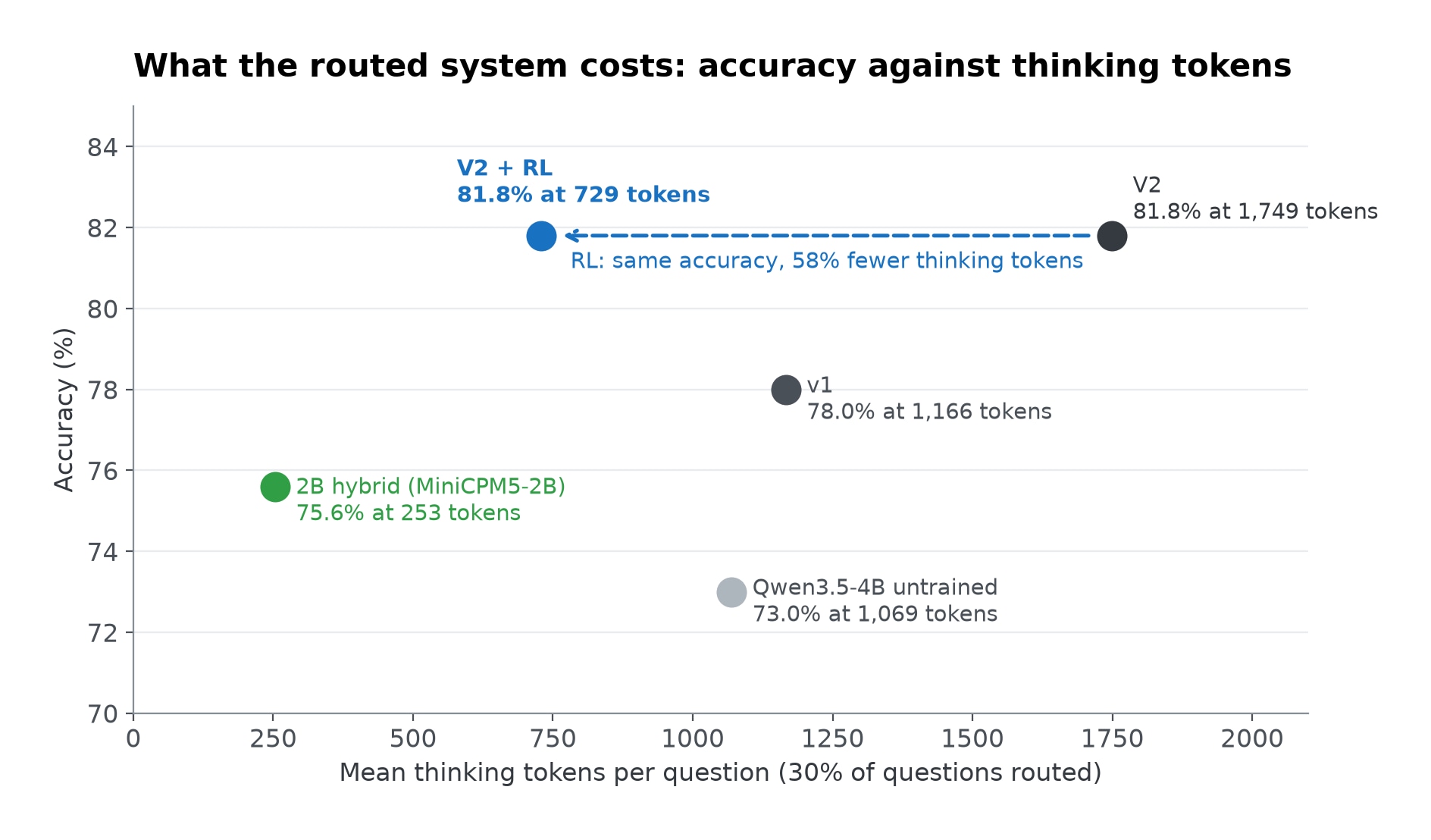
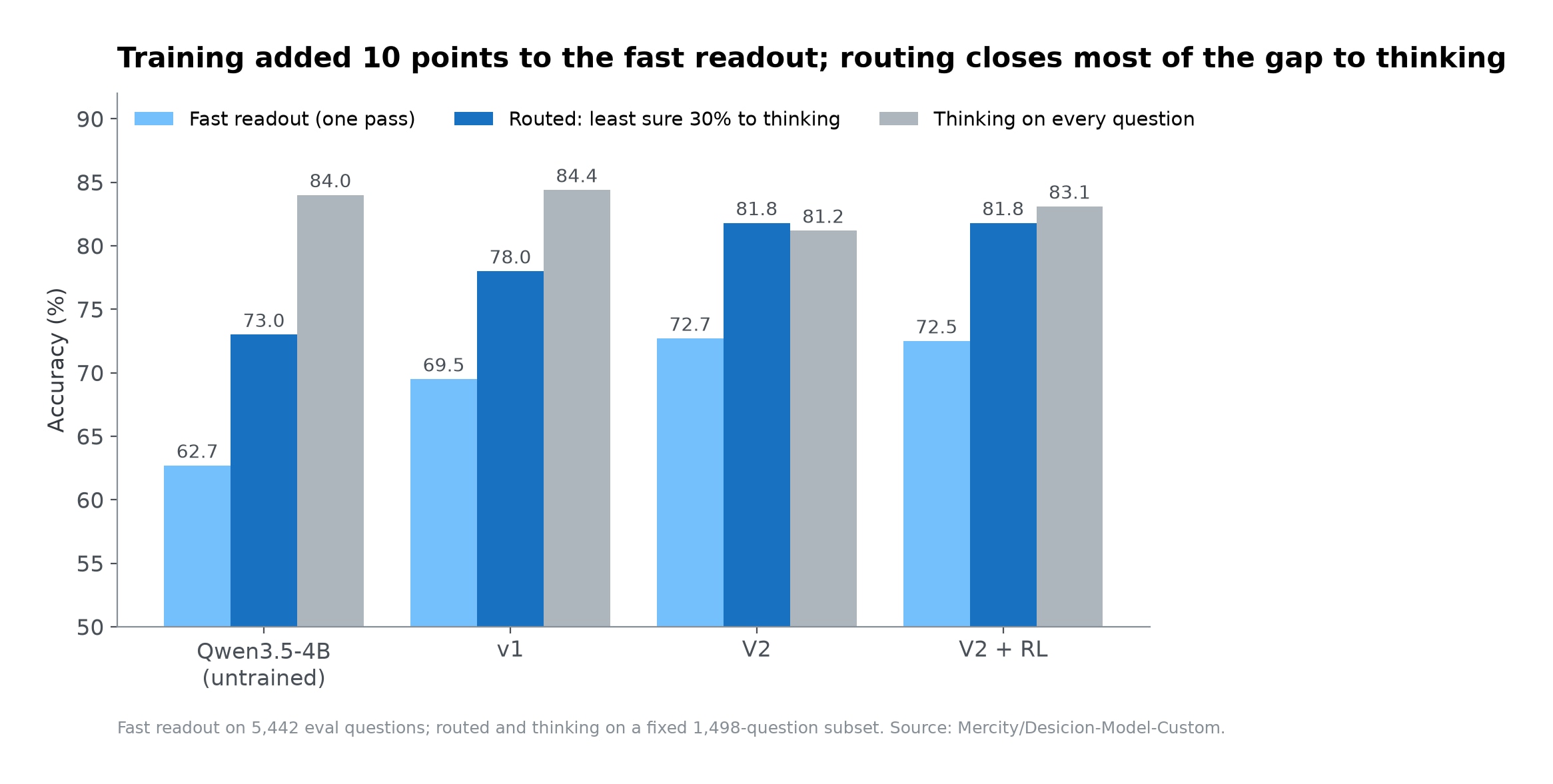
TRL’s default importance-sampling correction zeroed out most long chains and cost us a round, until we switched to per-token truncation. After that, 60 steps were enough: looping fell from 5.1% to 0.2%, thinking accuracy recovered to 83.1%, thinking tokens fell by more than half, and “Wait”s per chain dropped from about 10 to 5. Only 49% of RL questions gave useful signal, because many were solved by all 8 chains, so next time we would pick questions thinking mode solves 30 to 70% of the time.
Step 6: Route Only the Questions the Model Is Unsure About
Thinking is still expensive, so the last step decides who gets it. The router ranks questions by margin, the gap between the log-probabilities of the top two options after the per-type temperatures from Step 4, and sends the smallest-margin share to thinking. The temperatures and the cutoff both come from calibration data, never from eval (simplified from metrics.py):
# Fitted once, on held-out calibration questions only
temps = {qt: fit_temperature(cal_logits[qt], cal_gold[qt])     # minimises NLL
         for qt in ("choice", "noul", "score")}
cutoff = margin_that_routes(cal_questions, share=0.30)

# At serving time
p = softmax(fast_logits / temps[q.type])
top1, top2 = sorted(log(p), reverse=True)[:2]
if top1 - top2 >= cutoff:
    answer = argmax(p)                         # confident: fast readout
else:
    answer = think(q) or argmax(p)             # unsure: think; a looped chain falls back
That simple rule held up, since a learned router we trained did not beat it. At 30% routed the final model reaches 81.8%, matching the pre-RL model at 42% of its thinking budget, and 50% routed gave only 82.2%. That flat curve makes the routing share the main cost dial, so plot it on your own data before picking a number.
What Our Decision Model Results Showed
Together, the six steps added 10 points to the fast readout, from 62.7% for the untrained Qwen3.5-4B to 72.5%, and routing brought the system to within 1.3 points of thinking on every question. We put 95% paired-bootstrap intervals on every comparison, and they are all in the bucket.
Gains Shrink as Data Moves Away From Training
Those averages hide a wide spread. Procedural questions jumped from 46.8% to 89.5%, while real-world LocalLLaMA decisions, the set least like our training data, moved only from 63.0% to 66.3%. Part of that gap is label noise: on LocalLLaMA, 55 of the 141 thinking errors picked an option whose annotator share was within 0.15 of the gold answer.
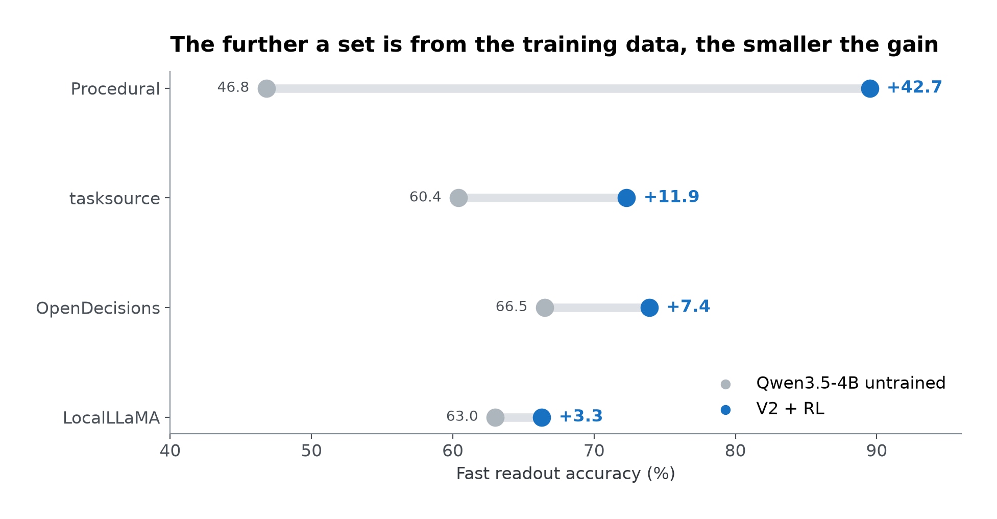
A model trained on generated data looks excellent on similar data and only modestly better on messy real traffic, so add diverse real sources rather than more questions from the same generators.
Thinking Wins by Computing
The same spread shows where thinking helps: when the answer needs explicit work. Thinking lifted OpenDecisions from 77% to 96%, and in 21 of the 30 fixes we read by hand, the chain did sums, date checks, counts, table joins or rule-by-rule checks. On judgment-heavy sets it broke about as many answers as it fixed (56 breaks against 60 fixes on LocalLLaMA).
That pattern says where to spend thinking: routing by task type as well as margin, so calculation-style decisions think even when the readout is confident, could reach 84.1% at the same budget on our eval.
Results on Outside Benchmarks
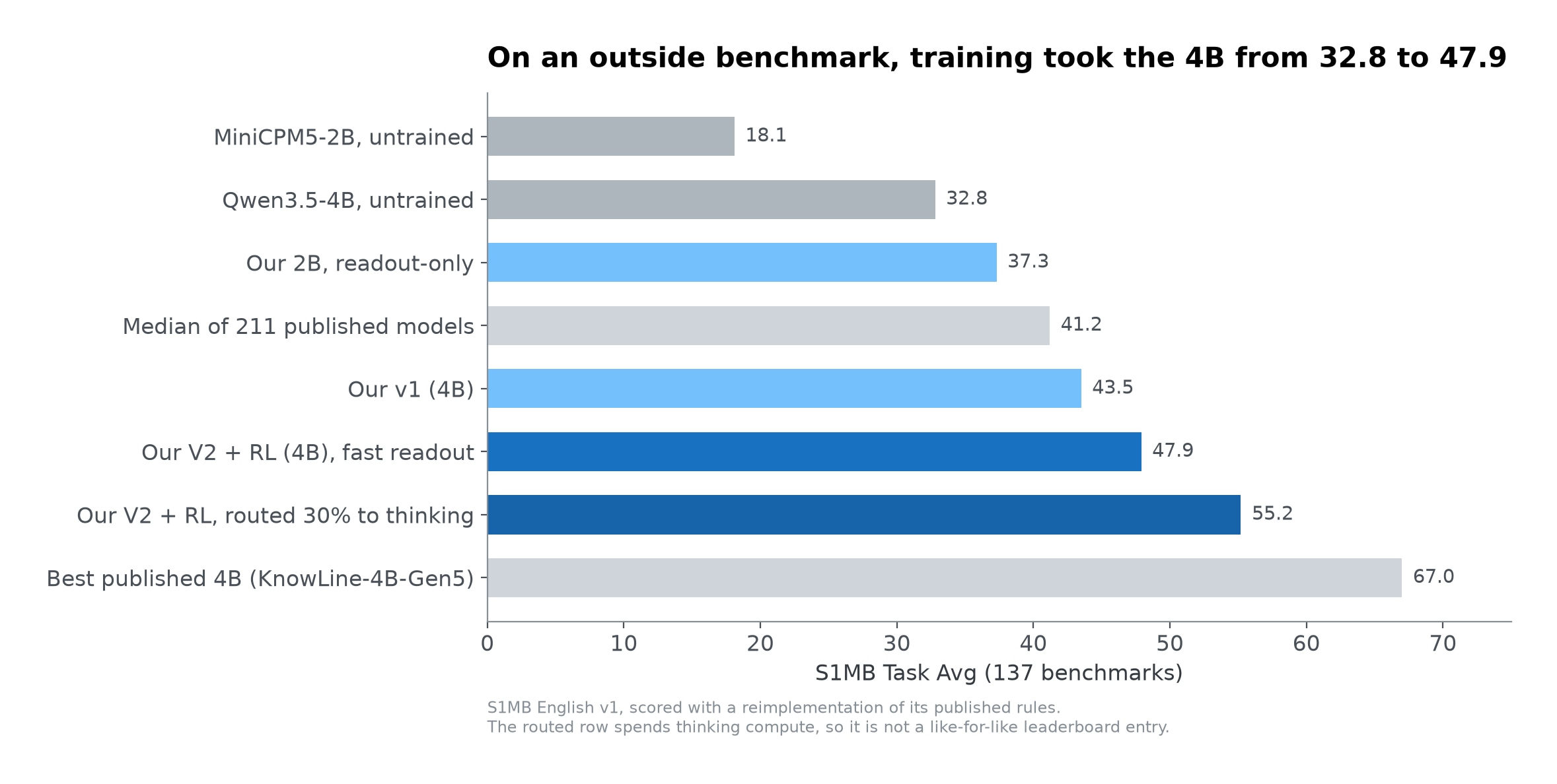
Our own eval could flatter us, so we checked outside ones. On S1MB, a benchmark of 137 tasks with 211 published models, training raised our Task Avg from 32.8 to 47.9, and 55.2 with routing. Gains were larger on benchmarks from datasets we never trained on (+17.4 against +8.4), so they are not memorization. On Jevals, the fast readout sits mid-pack, 6 to 10 points behind Jev, but it is among the best calibrated models on the board.
The recipe transfers down a size with one twist. On a 2B version built on MiniCPM5-2B, every fine-tune damaged thinking by 8 to 9 points, so the working 2B uses the trained adapter for fast answers and switches it off for thinking. That hybrid reaches 75.6% at 30% routed with only 253 thinking tokens per question, which makes it the better choice where GPU memory is tight.
How to Evaluate a Decision Model Before It Ships
Leaderboards are where most evaluation starts, and they disagree with each other. Depending on the board and the week, the top spot has belonged to GLiDE, StartLux, Clef or vLLM Semantic Router’s d3, and many headline numbers are self-reported runs on public subsets. Community efforts like the Decision Index reproduction kit and the Jev Atlas help, but none of them measures your policies.
That gap is why the eval that matters is built from real decisions your team has made. Measure calibration as well as accuracy on it, compare models with a paired bootstrap on the same questions to know whether a 1-point gain is real, and read outputs by hand, which is how we found that chains guessing at dataset conventions were right only 53 to 57% of the time, against about 90% for the rest. We wrote a longer guide on building custom evals for LLMs.
Offline evals still miss live traffic, so run the model in shadow mode before it blocks anything, logging its decisions next to what actually happened. If your decisions face customers, Heckler can generate the conversations to test it against.
Cost, Infrastructure and Compliance in Production
Once a model passes those checks, running it is cheap. The whole project, with both model sizes, all ablations, RL and every benchmark, took about 33 hours on one A100 80GB plus $6.60 in API calls, and the fast readout runs on vLLM with output restricted to the option letters, so it shares the stack you use for other models. From there, three things decide running cost:
- The routing share. Each routed question costs hundreds of thinking tokens. On our eval, going from 30% to 50% routed added only 0.4 points.
- Generation caps. A chain looping to 32K tokens is pure waste, so cap generation and fall back to the fast answer.
- Recalibration. Temperatures and thresholds drift when your traffic changes. Refit them on fresh held-out data whenever your policies or inputs shift.
The chains that cost money in routing also make compliance easier. Enterprises want a reason attached to a decision, and a bare probability is hard to defend to a customer or auditor. Thinking mode writes a chain for exactly the hardest cases, so log the state, the probabilities and the chain for every routed decision, and keep a person in the loop for decisions below your confidence threshold.
Want a Decision Model Trained on Your Own Decisions?
All of this happened in two months, as decision models went from one launch to an ecosystem with public recipes, and the change to the LLM can stay small: frozen weights, LoRA and a readout over your labels. What remains hard is the same as for any model: data that covers your real traffic, calibration you can trust, and evals built on your own decisions.
That is the work we do at Mercity: building custom models, synthetic data and evals for product and enterprise teams. Everything from this project is in our Hugging Face bucket, both models are open weights (4B, 2B), and if you want a decision model trained on your own policies and data, talk to us.